From Google Earth
http://feedproxy.google.com/~r/GoogleEarthBlog/~3/bwqgIMa5N68/kite_photos_of_tikehau_island_now_i.html
Art Trembanis
CSHEL
Department of Geological Sciences
University of Delaware
http://cshel.geology.udel.edu
From Google Earth
http://feedproxy.google.com/~r/GoogleEarthBlog/~3/bwqgIMa5N68/kite_photos_of_tikehau_island_now_i.html
Art Trembanis
CSHEL
Department of Geological Sciences
University of Delaware
http://cshel.geology.udel.edu
Art Trembanis
CSHEL
Department of Geological Sciences
University of Delaware
http://cshel.geology.udel.edu
Art Trembanis
CSHEL
Department of Geological Sciences
University of Delaware
http://cshel.geology.udel.edu
Art Trembanis
CSHEL
Department of Geological Sciences
University of Delaware
http://cshel.geology.udel.edu
Art Trembanis
CSHEL
Department of Geological Sciences
University of Delaware
http://cshel.geology.udel.edu
Art Trembanis
CSHEL
Department of Geological Sciences
University of Delaware
http://cshel.geology.udel.edu
Art Trembanis
CSHEL
Department of Geological Sciences
University of Delaware
http://cshel.geology.udel.edu
Northwestern University professor Malcolm MacIver's GhostBot is a robotic fish that can swim forward, backward, and vertically using its incredible ribbon-like fin. Ghostbot's locomotion is inspired by a knifefish in MacIver's aquarium, which a colleague observed making an unexpected, vertical movement.
Further observations revealed that while the fish only uses one traveling wave along the fin during horizontal motion (forward or backward depending on the direction on the wave), while moving vertically it uses two waves. One of these moves from head to tail, and the other moves tail to head. The two waves collide and stop at the center of the fin.
[via Neatorama]
Read the Full Story » | More on MAKE » | Comments » | Read more articles in Robotics | Digg this!
Art Trembanis
CSHEL
Department of Geological Sciences
University of Delaware
http://cshel.geology.udel.edu
Art Trembanis
CSHEL
Department of Geological Sciences
University of Delaware
http://cshel.geology.udel.edu
Art Trembanis
CSHEL
Department of Geological Sciences
University of Delaware
http://cshel.geology.udel.edu
From Google Earth
http://feedproxy.google.com/~r/GoogleEarthBlog/~3/osxtr7D_G_s/flooding_google_earth.html
Art Trembanis
CSHEL
Department of Geological Sciences
University of Delaware
http://cshel.geology.udel.edu

MAKE contributor James Floyd Kelly wrote in with a tip on a cool resource:
Found some GREAT information on Bolt Depot's homepage, including this printable poster that displays all the different bolts and nuts and connectors along with their official names. Click on the Fastener Tab at the top of the website and there are even more resources, including a great tutorial explaining how fasteners are identified (including how to accurately describe a bolt's length, type, etc.)Read the Full Story » | More on MAKE » | Comments » | Read more articles in Modern Mechanix | Digg this!

Girl, 10, becomes youngest to discover supernova...
A 10-year-old Canadian girl will head back to school this month with a good case for some extra credit in science: She became the youngest person to discover a supernova during the holiday break. Kathryn Aurora Gray of Fredericton, New Brunswick, spotted the exploding star, dubbed supernova 2010lt, on Monday from an image taken on New Year's Eve by a telescope belonging to amateur astronomer David Lane in Stillwater Lake, Nova Scotia. The exploding star is in the galaxy UGC 3378 in the constellation of Camelopardalis. The Royal Astronomical Society of Canada (RASC) says Kathryn is the youngest person ever to discover a supernova.If this sounds like fun to you - visit Galaxy Zoo and you could do this too!

Your task in this latest Galaxy Zoo project is to help us catch exploding stars – supernovae. Data for the site is provided by an automatic survey in California, at the world-famous Palomar Observatory, and astronomers are ready to follow up on your best candidates at telescopes around the world.Believe it or not humans are still better at picking out supernovae in photos than computers! Read the Full Story » | More on MAKE » | Comments » | Read more articles in Imaging | Digg this!
If you're looking for a way to fill up some of your after school time in the next few months, check out Google Science Fair. You can work solo or gather up a friend or two and set out to explore science and making while creating an online record of your project and process. You'll be competing against teens worldwide, but hey, the prizes look worthwhile.
Aged out of the competition? You can help out a team of youth as a teacher or mentor.
Check out the Maker Shed for some great information resources and hardware that might help your project.
Read the Full Story » | More on MAKE » | Comments » | Read more articles in Education | Digg this!
Art Trembanis
CSHEL
Department of Geological Sciences
University of Delaware
http://cshel.geology.udel.edu
![]()
![]()
Read more of this story at Slashdot.
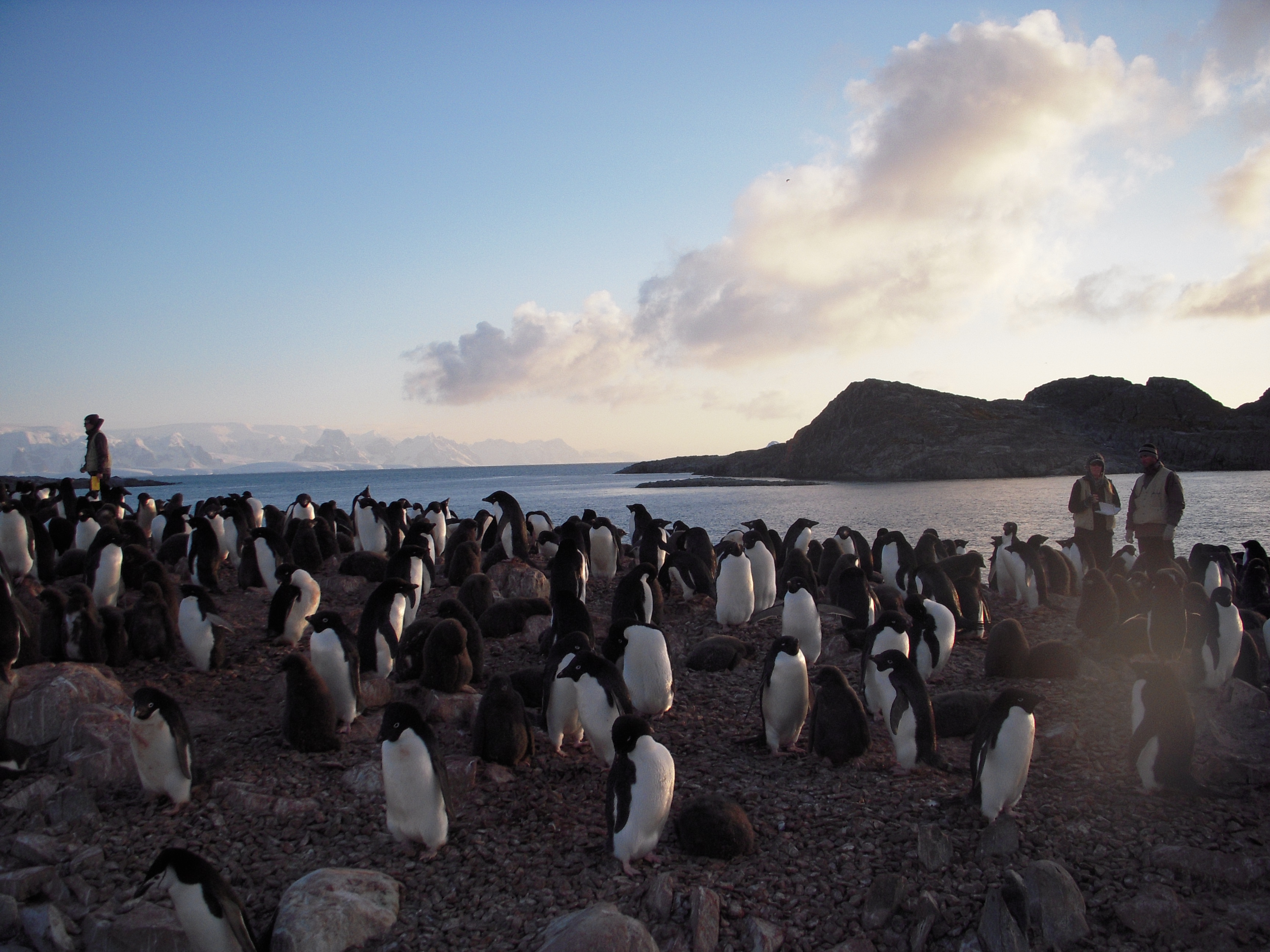
Adelie Penguin Rookery on Humble Island
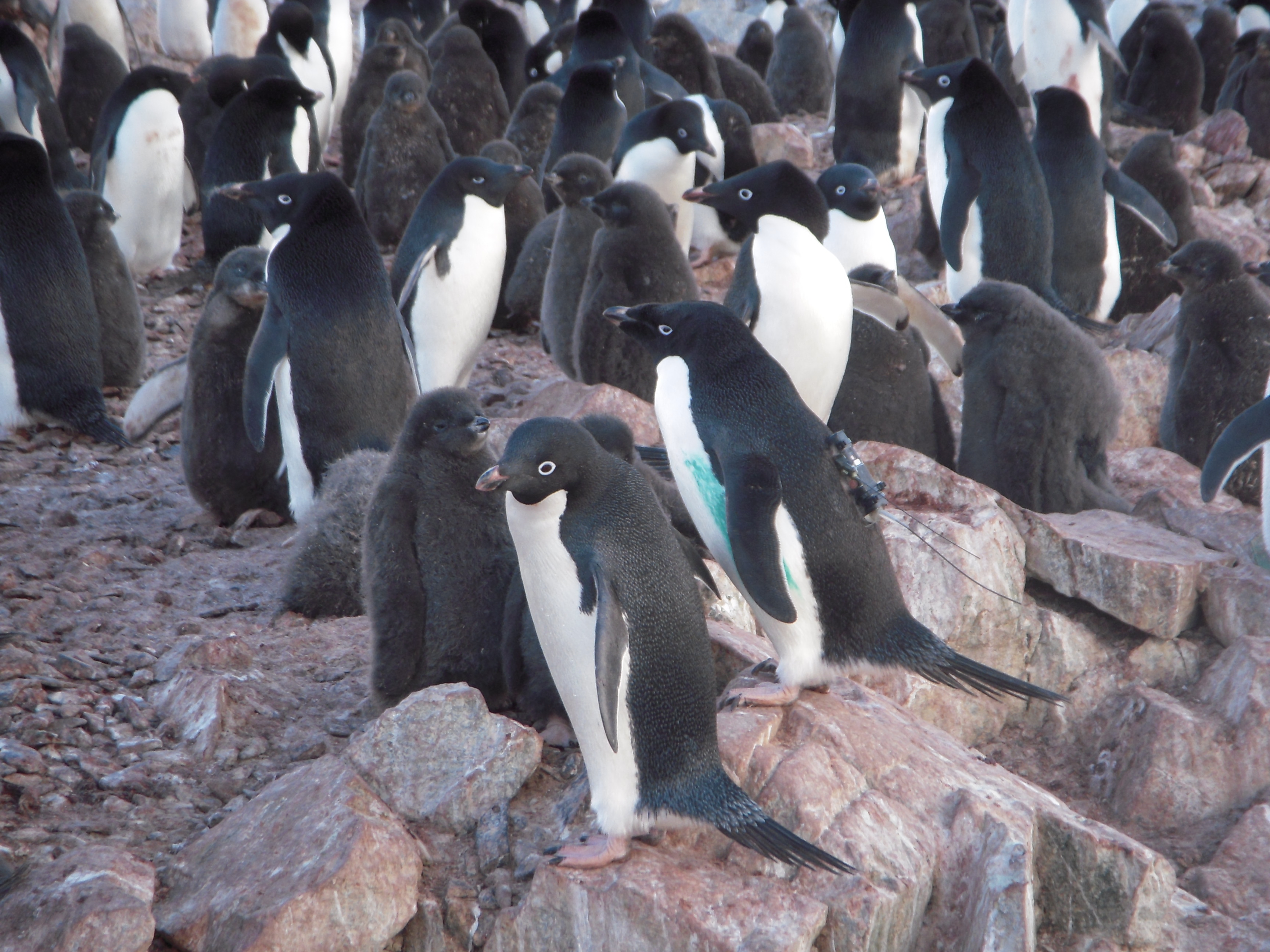
Satellite tagged Adelie Penguin

Penguin swimming tracks near Palmer Station
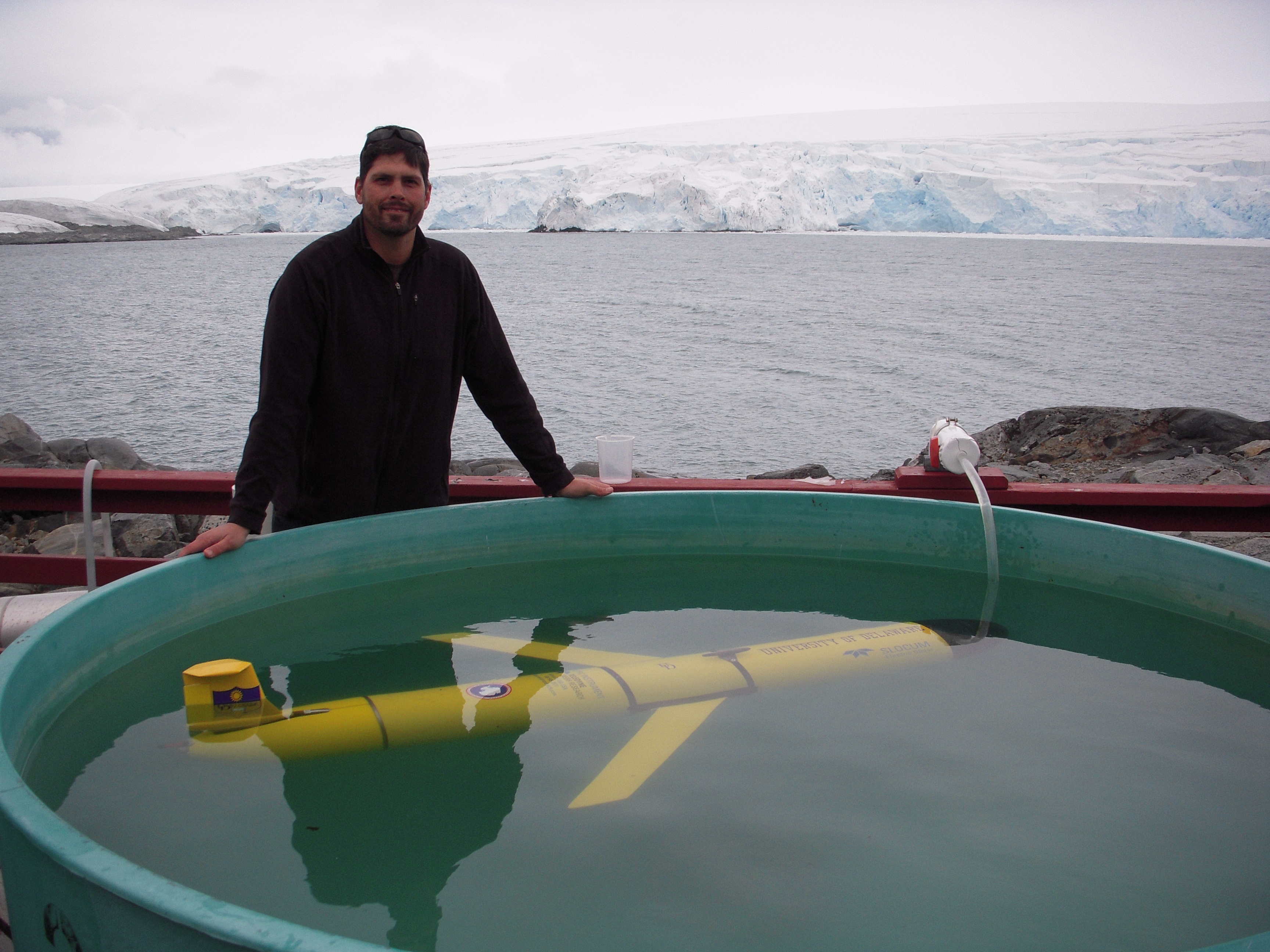
Ballasting the Glider (Blue Hen)
Is it possible to follow penguins from space to understand where and how they are feeding in Antarctica? Absolutely!..but not without an excellent team from University of Delaware, Rutgers University, Polar Oceans Research Group, and Cal Poly San Luis Obispo. The sequence starts with the "Birders". The "Birders" are from Polar Ocean Research and they have been studying penguins in the West Antarctic Peninsula for years. The "Birders", headed by Bill and Donna Fraser, head out to local rookeries to identify good penguins to tag with satellite transmitters. Finding the right breeding pair is key. The pair should have two chicks with both parents still around. Some chicks only have one parent, probably because one parent was killed by a Leopard Seal. We want to choose one of the parents, because we are pretty certain they will return to their chicks to feed them. This also helps in recovering the transmitter. If the bird does not return, the transmitter comes off during their natural annual molt cycle. Once a penguin is selected, it is gently fitted with a satellite transmitter. Special waterproof tape is used to connect the transmitter to the thick feathers on the back of the penguin. The penguins are remarkably calm during the process. Once the tag is attached, the penguin is released back to its nest. The next part of the sequence is for the birds. The penguins head out to feed on krill and small fish in the area. Their tags relay their position information to ARGOS satellites and we get nightly updates. The Birders pass on their data to me nightly, and I filter and map the penguin tracks. I put them into Google Earth, so we can see where the penguins have been feeding. Then, through the magic of mathematics, we turn their tracks into predicted penguin densities. Based on these densities, we plan our AUV missions to intersect with the feeding penguins (Slocum Electric Gliders and REMUS AUV's). The first priority is to make sure the AUV's are ballasted correctly. This means that they need to be trimmed with weights just right so they travel correctly under the water. We use small balances and scales to get the weight of the vehicle just right, then put them into ballasting tanks to make sure we did it correctly. The vehicles should hold steady just under the surface of the water.
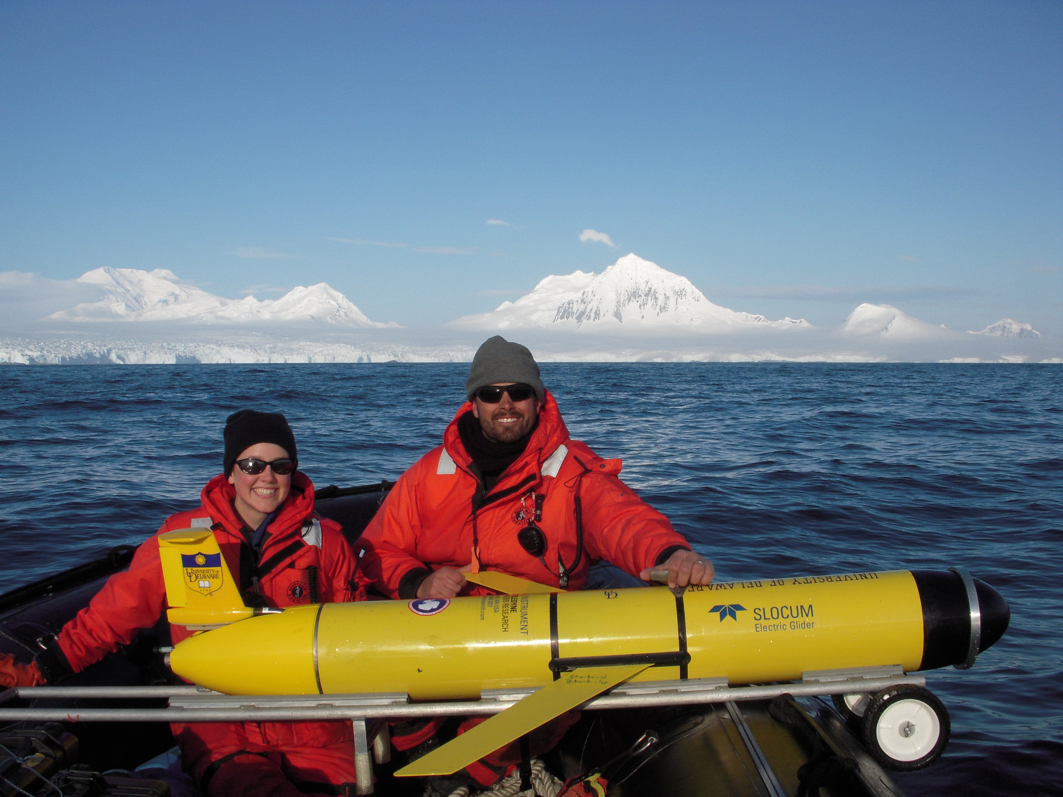
Getting ready for the launch of the "Blue Hen" (M. Oliver and K. Coleman)
Once we have a planned mission, we head out in small zodiacs from the station to a pre-determined point. For the Gliders, we call mission control at Rutgers University (Dave, Chip, John) and let them know a glider will be in the water shortly. Once it is in, control of the glider is accomplished via satellite telephone directly to the glider. The glider calls in and reports data and position to mission control. We can see the data coming in live over the web, and in Google Earth as we navigate the vehicle to where the penguins are feeding. The gliders move by changing their ballast, which allows them to glide up and down in the water while their wings give them forward momentum. They "fly" about 0.5mph for weeks at a time!
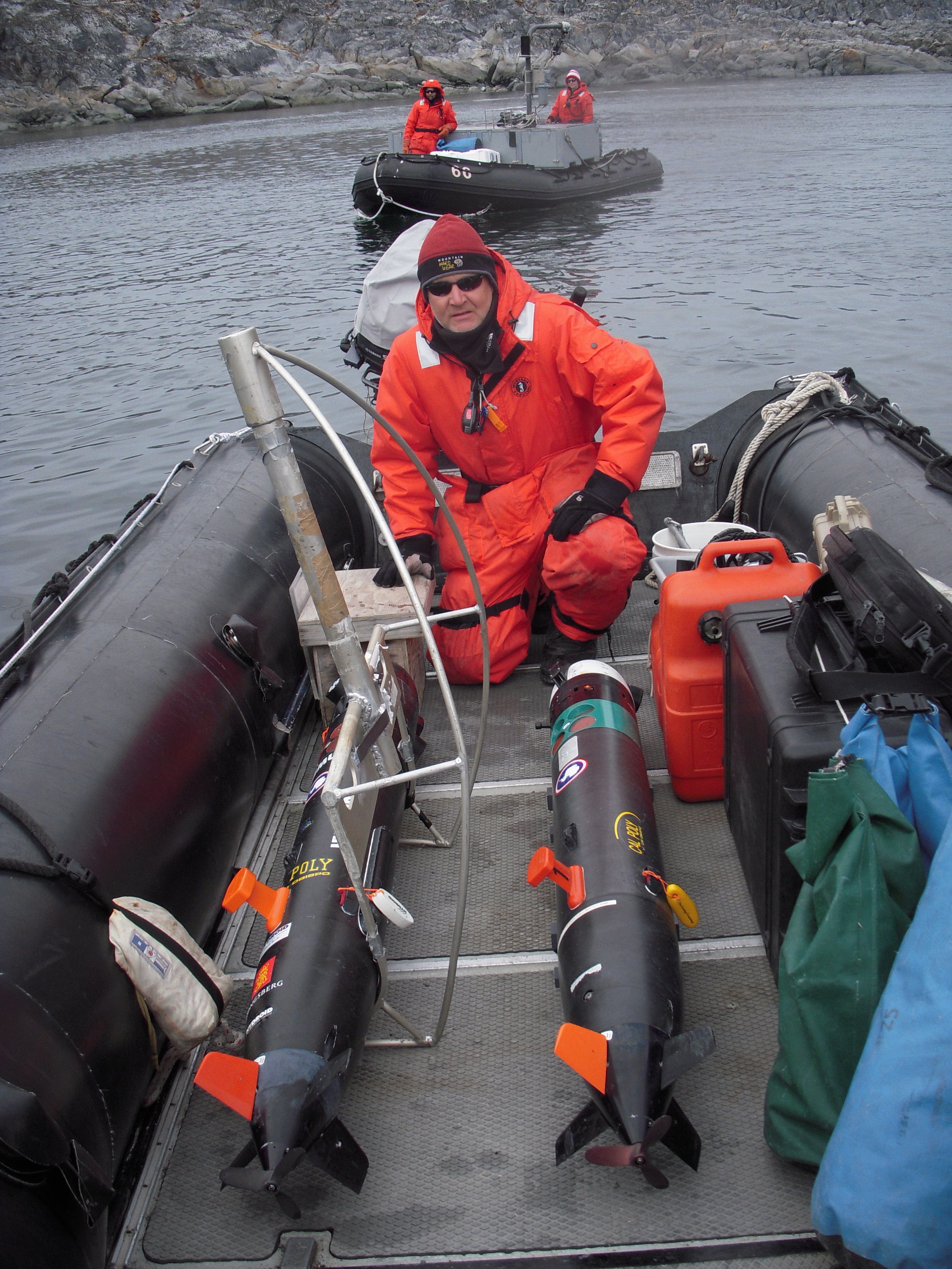
Mark Moline with REMUS's
In contrast to the Gliders, the REMUS vehicles are very fast and are designed for shorter, 1 day missions. Daily missions are planned around the penguin foraging locations. The Cal Poly Group (Mark Moline and Ian Robbins) have been launching 2 Remus Vehicles per day to map areas the gliders can't get too. Like the gliders, these vehicles call back via iridium to let us know how they are doing in their mission.
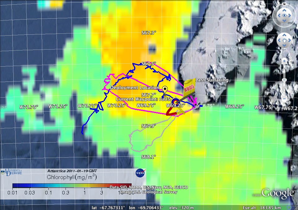
Glider Dances around Adelie Penguin Tracks in a sea of chlorophyll
Finally, we are getting satellite support from my lab at U.D. Erick, Megan and Danielle have been processing temperature and chlorophyll maps in near-real time to support our sampling efforts, as well as AUV operations up and down the West Antarctic Peninsula. Just today, we saw that the penguins in Avian Island (south by a few hundred miles) have been keying off of a chlorophyll front. RU05 was deployed by the L. M. Gould and will be recovered soon. All in all, it is a pretty awesome mission to track these penguins from space and AUV's. We will see how the season develops!
Guest blogger, Kelly Luetkemeyer, who is a Mapping Toolbox software developer at The MathWorks, returns with another article about using and analyzing data obtained from a Web Map Service (WMS) server.
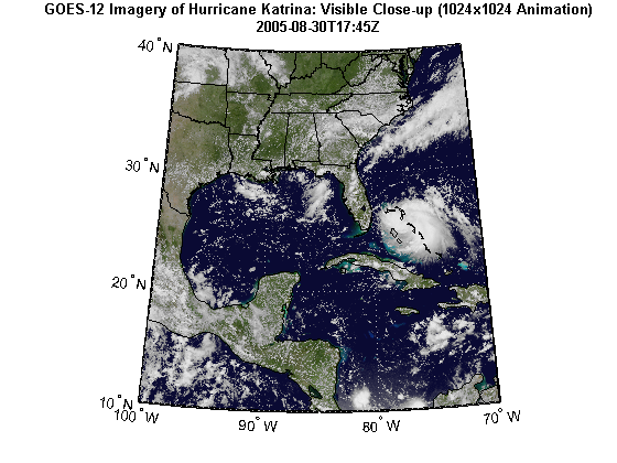
This demo shows how to track a hurricane using data from a WMS server. Typically web sites containing weather imagery may contain a visual animation of GOES imagery for any given hurricane. For example, a typical time-sequenced imagery of Katrina from a web site hosting weather imagery is shown below in an animated GIF.
Note that this animation shows the data in an unprojected geographic coordinate system. However, you may wish to view the data in a projected coordinate system, and overlay the hurricane track and the size of the hurricane, at any given point in time.
You can use MATLAB® to analyze images from a WMS server and track a hurricane's position and area. This demo will show you how to obtain the WMS imagery from a web site using features from the Mapping Toolbox™, analyze the imagery using features from the Image Processing Toolbox™, and use parfor from the Parallel Computing Toolbox™ to parallelize some computations for performance improvements.
In particular, this demo will show you how to:
The hurricane layer is from the NASA Goddard Space Flight Center's Scientific Visualization Studio (SVS) Image Server. The data in this layer shows cloud patterns in the visible wavelength, from 0.52 to 0.72 microns, during hurricane Katrina from August 24 through August 30 2005. The cloud data was extracted from the Geostationary Operational Environment Satellite (GOES-12) imagery and overlaid on a background color image of the southeast United States.
Since WMS servers are located on the Internet, this demo can be set to access the Internet to dynamically render and retrieve the maps from the WMS server or it can be set to use data previously retrieved from the Internet using the WMS capabilities but now stored in local files.
If you are new to WMS, several key concepts are important to understand and are listed here.
The code shown in this demo can be found in this function:
function track_hurricane(useInternet)This demo creates or reads several data files from a directory and uses the variable datadir to denote their location.
datadir = fullfile(pwd, 'KatrinaData'); if ~exist(datadir, 'dir') mkdir(datadir) end
Define an anonymous function to prepend datadir to the input filename:
datafile = @(filename)fullfile(datadir, filename);
This demo uses data obtained from a Web Map Server and thus requires Internet access. However, you can store the data locally the first time you run the demo and then set the useInternet flag to false. If the useInternet flag is not set, it defaults to false.
if ~exist('useInternet', 'var') useInternet = false; end
One of the more challenging aspects of using WMS is finding a WMS server and then finding the layer that is of interest to you. The process of finding a server that contains the data you need and constructing a specific and often complicated URL with all the relevant details can be very daunting.
The Mapping Toolbox™ simplifies the process of locating WMS servers and layers by providing a local, installed, and pre-qualified WMS database, that is search-able, using the function wmsfind. You can search the database for layers and servers that are of interest to you. Here is how you find layers containing the term katrina in either the LayerName or LayerTitle field of the database:
katrina = wmsfind('katrina'); whos katrina
Name Size Bytes Class Attributes katrina 95x1 47468 WMSLayer
The search for the term 'katrina' returned a WMSLayer array containing over 90 layers. To inspect information about an individual layer, simply display it like this:
katrina(1)
ans = WMSLayer Properties: Index: 1 ServerTitle: 'NASA SVS Image Server' ServerURL: 'http://aes.gsfc.nasa.gov/cgi-bin/wms?' LayerTitle: 'GOES-12 Imagery of Hurricane Katrina: Longwave Infrared Close-up (1024x1024 Animation)' LayerName: '3216_22510' Latlim: [15.0000 45.0000] Lonlim: [-100.0000 -70.0000]
If you type, katrina, in the command window, the entire contents of the array are displayed, with each element's index number included in the output. This display makes it easy for you to examine the entire array quickly, searching for a layer of interest. You can display only the LayerTitle property for each element by executing the command:
katrina.disp('Properties', 'layertitle', 'Index', 'off', 'Label', 'off');
As you've discovered, a search for the generic word 'katrina' returned results of over 90 layers and you need to select only one layer. In general, a search may even return thousands of layers, which may be too large to review individually. Rather than searching the database again, you may refine your search by using the refine method of the WMSLayer class. Using the refine method is more efficient and returns results faster than wmsfind since the search has already been narrowed to a smaller set.
Supplying the query string, 'goes-12*katrina*visible*close*up*animation', to the refine method returns a WMSLayer array whose elements contain a match of the query string in either the LayerTitle or LayerName properties. The * character indicates a wild-card search. You can use the first layer found.
katrina = katrina.refine('goes-12*katrina*visible*close*up*animation'); whos katrina
Name Size Bytes Class Attributes katrina 2x1 1032 WMSLayer
The database only stores a subset of the layer information. For example, information from the layer's abstract, details about the layer's attributes and style information, and the coordinate reference system of the layer are not returned by wmsfind. To return all the information, you need to use the wmsupdate function. wmsupdate synchronizes the layer from the database with the server, filling in the missing properties of the layer.
Synchronize the first katrina layer with the server and display the abstract information. Since this action requires access to the Internet, wrap the call around the useInternet flag.
cachefile = datafile('katrina.mat'); if useInternet katrina = wmsupdate(katrina(1)); if ~exist(cachefile, 'file') save(cachefile, 'katrina') end else load(cachefile) end
disp(['<html>' katrina.Abstract '</html>'])
The GOES-12 satellite sits at 75 degrees west longitude at an altitude of 36,000 kilometers over the equator, in geosynchronous orbit. At this position its Imager instrument takes pictures of cloud patterns in several wavelengths for all of North and South America, a primary measurement used in weather forecasting. The Imager takes a pattern of pictures of parts of the Earth in several wavelengths all day, measurements that are vital in weather forecasting. This animation shows a daily sequence of GOES-12 images in the visible wavelengths, from 0.52 to 0.72 microns, during the period that Hurricane Katrina passed through the Gulf of Mexico. At one kilometer resolution, the visible band measurement is the highest resolution data from the Imager, which accounts for the very high level of detail in these images. For this animation, the cloud data was extracted from GOES image and laid over a background color image of the southeast United States. Additional Credit: B>Please give credit for this item to:</b><br />
You can find out more information about the katrina layer by exploring the Details property of the katrina layer. The Details.Attributes field informs you that the layer has fixed width and fixed height attributes, thus the size of the requested map cannot be modified.
katrina.Details.Attributes
ans = Queryable: 0 Cascaded: 0 Opaque: 1 NoSubsets: 1 FixedWidth: 1024 FixedHeight: 1024
The Details.Dimension field informs you that the layer has a time dimension
katrina.Details.Dimension
ans = Name: 'time' Units: 'ISO8601' UnitSymbol: '' Default: '2005-08-30T17:45Z' MultipleValues: 0 NearestValue: 0 Current: 0 Extent: '2005-08-23T17:45Z/2005-08-30T17:45Z/P1D'
with an extent from 2005-08-23T17:45Z to 2005-08-30T17:45Z with a period of P1D (one day), as shown in the Details.Dimension.Extent field.
katrina.Details.Dimension.Extent
ans = 2005-08-23T17:45Z/2005-08-30T17:45Z/P1D
Since the layer has a time dimension, you can extract the time extent.
extent = katrina.Details.Dimension.Extent; slash = '/'; slashIndex = strfind(extent, slash); startTime = extent(1:slashIndex(1)-1); endTime = extent(slashIndex(1)+1:slashIndex(2)-1);Calculate numeric values for the start and end days. Note that the time extent is in yyyy-mm-dd format.
hyphen = '-'; hyphenIndex = strfind(startTime, hyphen); dayIndex = [hyphenIndex(2) + 1, hyphenIndex(2) + 2]; startDay = str2double(startTime(dayIndex)); endDay = str2double(endTime(dayIndex));The hurricane is not well-formed on the first day so start on the next day.
startDay = startDay + 1;
Create a requestTime variable to contain the start date.
requestTime = startTime; requestTime(dayIndex) = num2str(startDay);
Now that you have found a layer of interest, you can retrieve the raster map using the function wmsread and display the map using the function geoshow. You can specify the requested time by setting the Time optional parameter.
cachefile = datafile('katrina.tif'); if useInternet [katrinaMap, R] = wmsread(katrina, 'Time', requestTime); if ~exist(cachefile, 'file') imwrite(katrinaMap, cachefile) worldfilewrite(R, getworldfilename(cachefile)) end else katrinaMap = imread(cachefile); R = worldfileread(getworldfilename(cachefile)); end
Display the katrinaMap and overlay the outlines of land areas worldwide and the United States using data from shape files shipped with the Mapping Toolbox™.
states = shaperead('usastatehi.shp', 'UseGeoCoords', true); land = shaperead('landareas.shp', 'UseGeoCoords', true); figure('Color', 'white', 'Renderer', 'zbuffer') usamap(katrina.Latlim, katrina.Lonlim) geoshow(katrinaMap, R) geoshow(states, 'FaceColor', 'none') geoshow(land, 'FaceColor', 'none') title({katrina.LayerTitle, katrina.Details.Dimension.Default}, ... 'Interpreter', 'none', 'FontWeight', 'bold');
Using the imagery from the WMS server, calculate the hurricane's area and location of the center by assuming that the hurricane is in the region with the most cloud cover (as defined in pixel units, not map units).
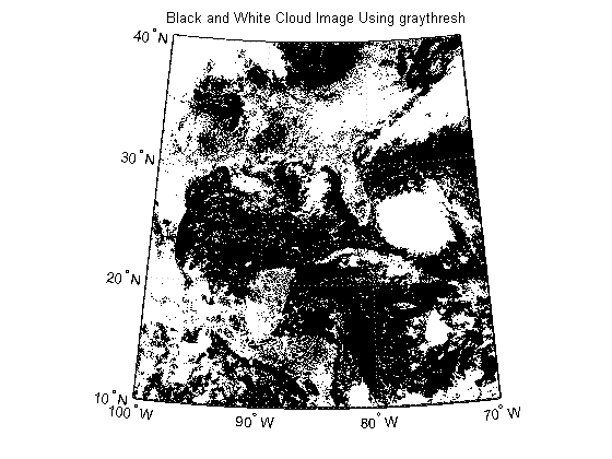
The first step is to create a black and white image from the image of Katrina. As an initial guess, try using the graythresh function to calculate a threshold value.
thresh = graythresh(katrinaMap); katrina_bw = im2bw(katrinaMap, thresh); figure('Color', 'white', 'Renderer', 'zbuffer') usamap(katrina.Latlim, katrina.Lonlim) geoshow(katrina_bw, R) title('Black and White Cloud Image Using graythresh')
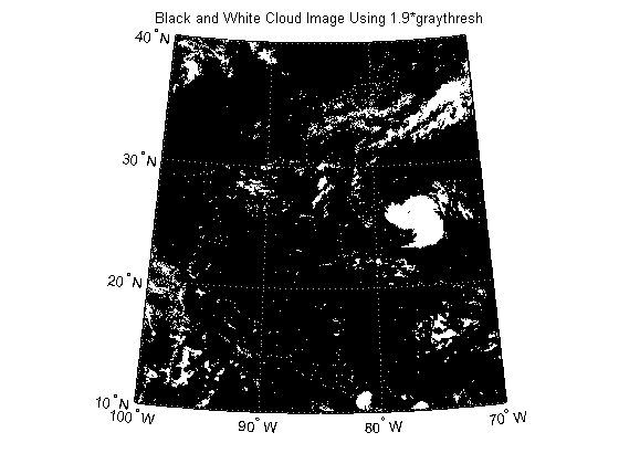
In the black and white image, you can see that there exists large tracts that are now white even though these areas do not have significant cloud cover. One method to remove these regions is to set a higher threshold value.
factor = 1.9; thresh = factor*thresh; katrina_bw = im2bw(katrinaMap, thresh); figure('Color', 'white', 'Renderer', 'zbuffer') usamap(katrina.Latlim, katrina.Lonlim) geoshow(katrina_bw, R) title('Black and White Cloud Image Using 1.9*graythresh')
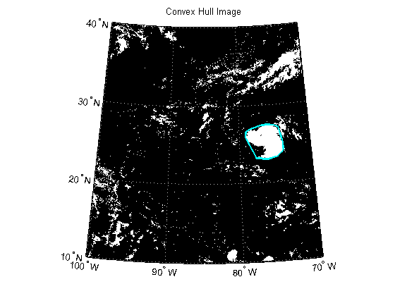
Calculate the convex hulls and areas of all regions using regionprops.
katrina_props = regionprops(katrina_bw, {'ConvexHull', 'Area'});Find the index that outlines the maximum area (in pixel units).
[~, maxIndex] = max([katrina_props(:).Area]); maxIndex = maxIndex(1);
Convert the row and column indices where the area is at a maximum to latitude and longitude coordinates. Store the coordinates into a structure.
row = katrina_props(maxIndex).ConvexHull(:,2); col = katrina_props(maxIndex).ConvexHull(:,1); ConvexHull = struct('Lat', [], 'Lon', [], 'Area', []); [ConvexHull.Lat, ConvexHull.Lon] = pix2latlon(R, row, col);
Plot the convex hull onto the black and white cloud image.
figure('Color', 'white', 'Renderer', 'zbuffer') usamap(katrina.Latlim, katrina.Lonlim) geoshow(katrina_bw, R) geoshow(ConvexHull.Lat, ConvexHull.Lon, 'Color', 'cyan', 'LineWidth', 2) title('Convex Hull Image')
Calculate the area of the convex hull in units of square statute miles.
ellipsoid = almanac('earth','wgs84','statutemiles'); ConvexHull.Area = areaint(ConvexHull.Lat, ConvexHull.Lon, ellipsoid);
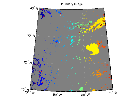
Calculate the boundaries of all objects using bwboundaries.
[B, L] = bwboundaries(katrina_bw);
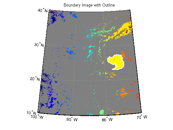
Convert the label matrix to an RGB image and display it.
labelRGB = label2rgb(L, @jet, [.5 .5 .5]); figure('Color', 'white', 'Renderer', 'zbuffer') usamap(katrina.Latlim, katrina.Lonlim) geoshow(labelRGB, R) title('Boundary Image')
Use a histogram to select the region with the most cloud cover.
clouds = L(L~=0); [freq, loc] = hist(clouds ,unique(L)); [~, maxIndex] = max(freq); hurricane = loc(maxIndex);
Capture indices of the largest cloud cover.
indices = B{hurricane}; row = indices(:,1); col = indices(:,2);Convert indices of the largest cloud cover to latitude and longitude.
Boundary = struct('Lat', [], 'Lon', [], 'Area', []); [Boundary.Lat, Boundary.Lon] = pix2latlon(R, row, col);
Plot the boundary onto the labeled image.
figure('Color', 'white', 'Renderer', 'zbuffer') usamap(katrina.Latlim, katrina.Lonlim) geoshow(labelRGB, R) geoshow(Boundary.Lat, Boundary.Lon, 'Color', 'white', 'LineWidth', 2) title('Boundary Image with Outline')
Calculate the area of the boundary in units of square statute miles.
Boundary.Area = areaint(Boundary.Lat, Boundary.Lon, ellipsoid);
Find the center of the hurricane.
katrina_center = regionprops(L, 'Centroid'); center_row = katrina_center(hurricane).Centroid(:,2); center_col = katrina_center(hurricane).Centroid(:,1); Centroid = struct('Lat', [], 'Lon', []); [Centroid.Lat, Centroid.Lon] = pix2latlon(R, center_row, center_col);
Import hurricane track vector data. The vector dataset, katrina.shp, contains the historical track for hurricane Katrina. The track file contains the 6-hourly (0000, 0600, 1200, 1800 UTC) center locations and intensities of the hurricane.
tracks = shaperead('KatrinaData/katrina.shp', 'UseGeo', true); tracks(1)
ans = Geometry: 'Line' BoundingBox: [2x2 double] Lon: [-75.1 -75.7 NaN] Lat: [23.1 23.4 NaN] Year: 2005 Month: 8 Day: 23 Name: 'KATRINA_2005' Wind_Knots: 30 Pressure: 1008 Cat: 'TD'
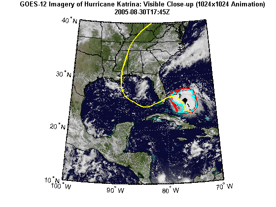
Display the WMS basemap and vector overlays:
figure('Color', 'white', 'Renderer', 'zbuffer') usamap(katrina.Latlim, katrina.Lonlim) geoshow(katrinaMap, R) geoshow(land, 'FaceColor', 'none') geoshow(states, 'FaceColor', 'none') geoshow(ConvexHull.Lat, ConvexHull.Lon, ... 'LineWidth', 4, 'Color', 'red'); geoshow(Boundary.Lat, Boundary.Lon, ... 'LineWidth', 2, 'Color', 'cyan'); geoshow(Centroid.Lat, Centroid.Lon, ... 'LineWidth', 4, 'Color', 'black', 'Marker', '+') geoshow(tracks, 'LineWidth', 2, 'Color', 'yellow') title({katrina.LayerTitle, katrina.Details.Dimension.Default}, ... 'Interpreter', 'none', 'FontWeight', 'bold');
Print the area statistics.
fprintf('Area of the convex hull is %0.2f square statute miles.\n', ... ConvexHull.Area); fprintf('Area of the boundary is %0.2f square statute miles.\n', ... Boundary.Area);
Area of the convex hull is 81463.28 square statute miles. Area of the boundary is 61953.07 square statute miles.
Now that you have developed an algorithm to track and calculate the hurricane's size and position, the next step is to apply that algorithm to a time sequence of data from the server. Use the parfor command to distribute the calculations to multiple processors. It is part of the MATLAB® language, and behaves essentially like a regular for-loop if you do not have access to the Parallel Computing Toolbox™ product.
Calculate the total number of animation frames.
numFrames = endDay - startDay + 1;
Assign the initial requestTime.
requestTime = startTime;
Initialize variables to hold the data calculated from each frame.
time = cell(numFrames, 1); S = struct('Lat', [], 'Lon', [], 'Area', []); ConvexHull = S; Boundary = S; ConvexHull(numFrames) = ConvexHull; Boundary(numFrames) = Boundary; Centroid = struct('Lat', [], 'Lon', []); Centroid(numFrames) = Centroid; frameName = datafile('frame_');
Check the status of the MATLAB® pool and determine if it is open. Use the MATLAB® pool to allow the body of the parfor loop to run in parallel.
poolSize = matlabpool('size'); if poolSize == 0 fprintf('The MATLAB pool is not open, the loop will run sequentially.'); else fprintf('Using %d workers.\n', poolSize); end
Using 4 workers.
For each day, from startDay to endDay, perform the following operations:
To create the animation frames, you can load the rendered data from each saved MAT-file and capture the data to an image. You need to do this operation outside of the parfor loop since each compute lab is started in a headless mode. By storing each rendered frame into a MAT-file within the parfor loop, you can improve performance since rendering the data into a Figure window from a MAT-file is a faster operation than the display operations for the vector and raster data.
tworkers = zeros(1, poolSize); tic; parfor k=1:numFrames tstart = tic; % Update currentDay. currentDay = startDay + k -1; % Assign time value for this frame. frameTime = requestTime; frameTime(dayIndex) = num2str(currentDay); time{k} = frameTime; % Get the WMS map from the server (or file) for this time period. cachefile = datafile(['katrina_' num2str(currentDay) '.tif']); if useInternet RGB = wmsread(katrina, 'Time', frameTime); if ~exist(cachefile, 'file') imwrite(RGB, cachefile); end else RGB = imread(cachefile); end % Calculate the convex hull, boundary, areas, and centroid using the % same threshold value as calculated for the first image. [ConvexHull(k), Boundary(k), Centroid(k)] ... = calculateRegionProperties(RGB, R, thresh); % Render the frame. hFig = figure('Color', 'white', 'Renderer', 'zbuffer'); renderFrame(frameTime, katrina, RGB, R, ... ConvexHull(k), Boundary(k), Centroid(k), land, states, tracks); % Save the rendered frame. hAxes = get(hFig, 'CurrentAxes'); frameFilename = [frameName num2str(k) '.fig']; hgsave(hAxes, frameFilename); close(hFig); % Save the workers elapsed time. tworkers(k) = toc(tstart); % Print statistics fprintf('\nFrame %d elapsed time: %4.8f\n', k, tworkers(k)); fprintf('Frame %d convex hull area: %0.2f.\n', ... k, ConvexHull(k).Area); fprintf('Frame %d boundary area: %0.2f.\n', ... k, Boundary(k).Area); end tloop = toc;
Frame 4 elapsed time: 17.75099091 Frame 4 convex hull area: 179144.66. Frame 4 boundary area: 113185.27. Frame 2 elapsed time: 19.09949585 Frame 2 convex hull area: 192105.82. Frame 2 boundary area: 114881.50. Frame 6 elapsed time: 25.17652566 Frame 6 convex hull area: 443757.43. Frame 6 boundary area: 303722.05. Frame 5 elapsed time: 26.48190417 Frame 5 convex hull area: 161777.52. Frame 5 boundary area: 137392.76. Frame 3 elapsed time: 18.83270332 Frame 3 convex hull area: 149839.57. Frame 3 boundary area: 108983.98. Frame 1 elapsed time: 18.44629997 Frame 1 convex hull area: 81463.28. Frame 1 boundary area: 61953.07. Frame 7 elapsed time: 15.59668967 Frame 7 convex hull area: 248729.73. Frame 7 boundary area: 199408.60.
You expect the total time of all the workers to be more than the loop time when the loop is executed in parallel.
fprintf('Total time for all workers: %4.8f\n', sum(tworkers)); fprintf('Total loop time: %4.8f\n', tloop);
Total time for all workers: 141.38460955 Total loop time: 43.90086599
An animation can be viewed in the browser when the browser opens an animated GIF file or an AVI video file. To create the animation frames of the WMS basemap and vector overlays, render the data from the saved graphics files, capture the rendered data into a frame structure, and save frame into either an array for the animated GIF file or to an AVI video file.
To share with others or to post to web video services, you can create an AVI video file containing all the frames using the VideoWriter class.
basename = 'wmstrack'; videoFilename = ['html/' basename '.avi']; if exist(videoFilename, 'file') delete(videoFilename) end writer = VideoWriter(videoFilename); writer.FrameRate = 1; writer.Quality = 100; writer.open;
For each frame, read the graphics from the cache file created in the body of the parfor loop, and display the WMS basemap and vector overlays. Capture each frame and store into the frames array. The loop cannot run in parallel since the video frames must be ordered.
hFig = figure('Color', 'white', 'Renderer', 'zbuffer'); for k=1:numFrames % Delete the previous frame. hAxes = get(hFig, 'CurrentAxes'); delete(hAxes) % Load the basemap and vector overlays into the axes. frameFilename = [frameName num2str(k) '.fig']; hgload(frameFilename); % Capture the current frame. shg frame = getframe(hFig); % Store the frame into the |animated| array for the GIF file. if k == 1 [animated, cmap] = rgb2ind(frame.cdata, 256, 'nodither'); animated(:,:,1,numFrames) = animated; else animated(:,:,1,k) = rgb2ind(frame.cdata, cmap, 'nodither'); end % Write the frame to the AVI file. writer.writeVideo(frame); end % Close the Figure window and AVI file. close writer.close;
Write the animated GIF file.
filename = [basename '.gif']; delayTime = 2.0; imwrite(animated, cmap, filename, 'DelayTime', delayTime, 'LoopCount', inf);
An animation can be viewed in the browser when the browser opens an animated GIF file.
web(filename)

headers = {'Time', 'Latitude', 'Longitude', ... 'Convex Hull Area', 'Boundary Area'}; makeTable(headers, time, [Centroid.Lat], [Centroid.Lon], ... [ConvexHull.Area], [Boundary.Area]); | Time | Latitude | Longitude | Convex Hull Area | Boundary Area |
| 2005-08-24T17:45Z | 25.399 | -76.144 | 81463.282 | 61953.066 |
| 2005-08-25T17:45Z | 25.913 | -79.282 | 192105.821 | 114881.500 |
| 2005-08-26T17:45Z | 23.568 | -82.217 | 149839.573 | 108983.980 |
| 2005-08-27T17:45Z | 23.680 | -84.421 | 179144.655 | 113185.267 |
| 2005-08-28T17:45Z | 26.285 | -88.482 | 161777.517 | 137392.758 |
| 2005-08-29T17:45Z | 34.192 | -87.477 | 443757.435 | 303722.052 |
| 2005-08-30T17:45Z | 37.301 | -85.280 | 248729.729 | 199408.599 |
The following wmstrack.avi video is generated and can be viewed using an external viewer.
dbtype makeTable1 function makeTable(headers, time, lat, lon, area1, area2) 2 %makeTable Make HTML table 3 % 4 % makeTable(headers, time, lat, lon, area1, area2) generates and displays 5 % (using disp) HTML to visualize a table of input values. HEADERS is a 6 % cell array of names for the top row. The values of the table are in the 7 % arrays, TIME, LAT, LON, AREA1, and AREA2. 8 9 % Copyright 2010-2011 The MathWorks, Inc. 10 11 header = ' '; 12 for k=1:numel(headers) 13 tableEntry = sprintf( ... 14 '<td align="center"> <b> %s </b></td>', ... 15 headers{k}); 16 header = [header tableEntry]; %#ok<AGROW> 17 end 18 header = ['<tr>' header '</tr>']; 19 20 table = ' '; 21 for k = 1:numel(time) 22 tableEntry = sprintf( ... 23 ['<tr>', ... 24 '<td align="right"> %s </td>', ... 25 '<td align="right"> %0.3f </td>', ... 26 '<td align="right"> %0.3f </td>', ... 27 '<td align="right"> %0.3f </td>', ... 28 '<td align="right"> %0.3f </td></tr>'], ... 29 time{k}, lat(k), lon(k), area1(k), area2(k)); 30 table = [table tableEntry]; %#ok<AGROW> 31 end 32 33 disp([ ... 34 '<html><table border=1 cellpadding=1>', ... 35 header, ... 36 table, ... 37 '</table></html>']); endThis function calculates the convex hull, BW boundary, area, and centroid properties of an RGB image.
function [ConvexHull, Boundary, Centroid] = ... calculateRegionProperties(RGB, R, thresh) % Calculate the convex hull and area of the objects in the RGB image. bw = im2bw(RGB, thresh); props = regionprops(bw, {'ConvexHull', 'Area'}); % Find the indices that outline the maximum area. [~, maxIndex] = max([props(:).Area]); % Convert the row and column indices where the area is at a maximum to % latitude and longitude coordinates. Store the coordinates into a % structure. row = props(maxIndex).ConvexHull(:,2); col = props(maxIndex).ConvexHull(:,1); ConvexHull = struct('Lat', [], 'Lon', [], 'Area', []); [ConvexHull.Lat, ConvexHull.Lon] = pix2latlon(R, row, col); % Calculate the area of the convex hull in units of square statute miles. ellipsoid = almanac('earth','wgs84','statutemiles'); ConvexHull.Area = areaint(ConvexHull.Lat, ConvexHull.Lon, ellipsoid); % Calculate the boundaries of all objects. [B, L] = bwboundaries(bw); % Use a histogram to select the largest region. objects = L(L~=0); [freq, loc] = hist(objects ,unique(L)); [~, maxIndex] = max(freq); largestRegion = loc(maxIndex); % Capture indices of the largest region. indices = B{largestRegion}; row = indices(:,1); col = indices(:,2); % Convert indices of the largest region cover to latitude and longitude. Boundary = struct('Lat', [], 'Lon', [], 'Area', []); [Boundary.Lat, Boundary.Lon] = pix2latlon(R, row, col); % Calculate the area of the boundary in units of square statute miles. Boundary.Area = areaint(Boundary.Lat, Boundary.Lon, ellipsoid); % Find the center of the largest region. center = regionprops(L, 'Centroid'); center_row = center(largestRegion).Centroid(:,2); center_col = center(largestRegion).Centroid(:,1); Centroid = struct('Lat', [], 'Lon', []); [Centroid.Lat, Centroid.Lon] = pix2latlon(R, center_row, center_col); end
function renderFrame(frameTime, layer, layerMap, R, ... ConvexHull, Boundary, Centroid, land, states, tracks)
% This function renders the frame data into a Figure window. usamap(layer.Latlim, layer.Lonlim) geoshow(layerMap, R) geoshow(land, 'FaceColor', 'none') geoshow(states, 'FaceColor', 'none') geoshow(ConvexHull.Lat, ConvexHull.Lon, 'LineWidth', 4, 'Color', 'red'); geoshow(Boundary.Lat, Boundary.Lon, 'LineWidth', 2, 'Color', 'cyan'); geoshow(Centroid.Lat, Centroid.Lon, 'LineWidth', 4, 'Color', 'k', 'Marker', '+') geoshow(tracks, 'LineWidth', 2, 'Color', 'yellow') title({layer.LayerTitle, frameTime}, 'Interpreter', 'none', 'FontWeight', 'bold');
Katrina Layer
The Katrina layer used in the demo is from the NASA Goddard Space Flight Center's SVS Image Server and is maintained by the Scientific Visualization Studio.
For more information about this server, run:
>> wmsinfo('http://aes.gsfc.nasa.gov/cgi-bin/wms?')usastatehi.shp
This vector dataset contains moderate-resolution outlines and names for the 50 United States plus the District of Columbia, stored in shapefile format with coordinates in latitude (Y) and longitude (X) in degrees. It is based on U.S. Census Bureau's TIGER thinned boundary files. The data file is shipped with the Mapping Toolbox™.
landareas.shp
This vector dataset contains low-resolution outlines of land areas worldwide, stored as polygons in shapefile format with coordinates in latitude (Y) and longitude (X) in degrees. The raw coordinate data were derived from the Digital Chart of the World (DCW) browser layer, published by U.S. National Geospatial-Intelligence Agency (NGA), formerly National Imagery and Mapping Agency (NIMA). The data file is shipped with the Mapping Toolbox™.
katrina.shp
This vector dataset contains the historical track for hurricane Katrina. The raw data were obtained from the atl_hurtrack.shp file from the National Oceanic and Atmospheric Administration Coastal Services Center. This Historical North Atlantic Tropical Cyclone Tracks file contains the 6-hourly (0000, 0600, 1200, 1800 UTC) center locations and intensities for all subtropical depressions and storms, extra-tropical storms, tropical lows, waves, disturbances, depressions and storms, and all hurricanes, from 1851 through 2009. These data are intended for geographic display and analysis at the national level, and for large regional areas. The data should be displayed and analyzed at scales appropriate for 1:2,000,000-scale data. No responsibility is assumed by the National Oceanic and Atmospheric Administration in the use of these data. The complete track data was downloaded from NOAA. The data file is not shipped with the Mapping Toolbox™.
As you can see here, I've used parfor to independently fetch and process each frame before constructing the final video. Is that technique something you might be able to take advantage of? Let us know here.
end
Get the MATLAB code (requires JavaScript)
Published with MATLAB® 7.11
Art Trembanis
CSHEL
Department of Geological Sciences
University of Delaware
http://cshel.geology.udel.edu
http://www.noaanews.noaa.gov/stories2011/20110119_exploration.html
Art Trembanis
CSHEL
Department of Geological Sciences
University of Delaware
http://cshel.geology.udel.edu
Art Trembanis
CSHEL
Department of Geological Sciences
University of Delaware
http://cshel.geology.udel.edu
IBM's Watson supercomputer won a practice round against Jeopardy champions Ken Jennings and Brad Rutter and raised a lot of questions about the capabilities of artificial intelligence.Watson, a four-year effort by IBM, was quicker on the draw, didn't fall prey to emotion and had a voice that could be confused for wayward computer Hal 9000 from the movie 2001: A Space Odyssey. For IBM, Watson is about tackling verticals and bringing hardware and analytics to the fore.
A fun quote from the article about Watson...
Rutter said Watson can be a bit overwhelming. Jennings and Rutter quipped about how computer capabilities are part of human advancement, but acknowledged that they were a bit uncomfortable. Jennings said he "didn't want technology to advance that far just yet." When John Kelly III, director of IBM Research reminded Jennings and Rutter that computer and human intelligence were at an intersection point and computing would only improve, Rutter quipped: "So we're all extinct."
If Watson beats us, like Deep Blue did - will we ever be able to see how? 10 years from now, ever? Shouldn't kids of today be tinkering with their own Deep Blue in a virtual machine? There's nothing magical about a super Chess computer or Google-like IBM interface for answering trivia questions but each time a human vs machine bout happens shouldn't there also be a time when we share how it's done so we can do it better, or come up with something that's a bigger challenge? Or figure out a question a computer will never be able to answer?
I know there will be some comments like "who cares!" but think about the people (and machines) 100 years from now, I'm betting both would want to know how this all happened. We have a unique opportunity to comment the fossil record /*
So before I end this plea to IBM, how about this - IBM, you bring Watson to Maker Faire bay Area 2011 in May, last year we had over 80,000 attend - think of all the next-generation scientists and engineers that will be there to inspire.
This post was automatically generated by Multivac
Previously:
IBM supercomputer '"Watson" to challenge "Jeopardy" stars.
Also check out the great video on Engadget.
Art Trembanis
CSHEL
Department of Geological Sciences
University of Delaware
http://cshel.geology.udel.edu

Our own Laura Cochrane writes:
Flickr user Khol made a geological layers cake, inspired by Tim Babb's "Geology" design on Threadless. It makes me think of the song "Dirt Made My Lunch."
[via CRAFT]
More:
Read the Full Story » | More on MAKE » | Comments » | Read more articles in Science | Digg this!This week Richard Willey from technical marketing will be guest blogging about nonparametric fitting.
This week's blog is motivated by a common question on MATLAB Central. Consider the following problem:
How can you generate a curve fit that best describes the relationship between X and Y? This question traditionally shows up in in two different guises:
In this week's blog, I'm going to show you a better way to solve this same problem how to use a combination of localized regression and cross validation.
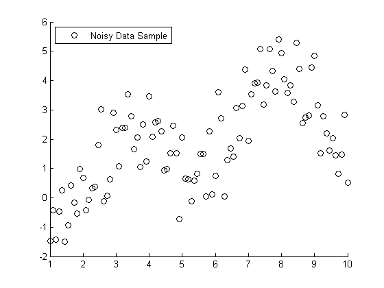
To use a more visual approach, suppose you had the following set of data points:
s = RandStream('mt19937ar','seed',1971); RandStream.setDefaultStream(s); X = linspace(1,10,100); X = X'; % Specify the parameters for a second order Fourier series w = .6067; a0 = 1.6345; a1 = -.6235; b1 = -1.3501; a2 = -1.1622; b2 = -.9443; % Fourier2 is the true (unknown) relationship between X and Y Y = a0 + a1*cos(X*w) + b1*sin(X*w) + a2*cos(2*X*w) + b2*sin(2*X*w); % Add in a noise vector K = max(Y) - min(Y); noisy = Y + .2*K*randn(100,1); % Generate a scatterplot scatter(X,noisy,'k'); L2 = legend('Noisy Data Sample', 2); snapnow
If you knew that this data was generated with a second order Fourier series, you use nonlinear regression to model Y = f(X).
foo = fit(X, noisy, 'fourier2') % Plot the results hold on plot(foo) L3 = legend('Noisy Data Sample','Nonlinear Regression', 2); hold off snapnow
foo = General model Fourier2: foo(x) = a0 + a1*cos(x*w) + b1*sin(x*w) + a2*cos(2*x*w) + b2*sin(2*x*w) Coefficients (with 95% confidence bounds): a0 = 1.734 (1.446, 2.021) a1 = -0.1998 (-1.065, 0.6655) b1 = -1.413 (-1.68, -1.146) a2 = -0.7688 (-1.752, 0.2142) b2 = -1.317 (-1.867, -0.7668) w = 0.6334 (0.5802, 0.6866)
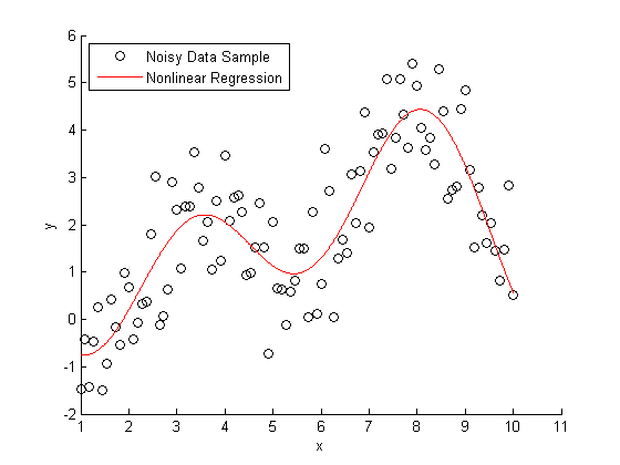
All very nice and easy... We were able to specify a regression model and plot our curve using a couple lines of code. The coefficients that were estimated by our regression model are a close match to the ones that we originally specified.
Here's the rub: we cheated. When we created our regression model, we specified that the true relationship between X and Y should be modeled using a second order Fourier series. What if this information wasn't available to us?
This next piece of code is a bit more complicated, however, it will solve the same problem using nothing but the raw data and some CPU cycles.
We're going to use a smoothing algorithm called LOWESS (Localized Scatter Plot Smoothing) to generate our curve fit. The accuracy of a LOWESS fit depends on specifying the "right" value for the smoothing parameter. We're going generate 99 different LOWESS models, using smoothing parameters between zero and one, and see which value generates the most accurate model.
This type of brute force technique often runs into problems with "overfitting". The LOWESS curve that minimizes the "sum of the squared errors" fits both the signal and the noise component of the data set.
To protect against overfitting, we're going to use a technique called cross validation. We're going to divide the data set into different training sets and test sets. We'll generate our predictive model using the data in the training set, and then measure the accuracy of the model using the data in the test set.
num = 99; spans = linspace(.01,.99,num); sse = zeros(size(spans)); cp = cvpartition(100,'k',10); for j=1:length(spans), f = @(train,test) norm(test(:,2) - mylowess(train,test(:,1),spans(j)))^2; sse(j) = sum(crossval(f,[X,noisy],'partition',cp)); end [minsse,minj] = min(sse); span = spans(minj);
mylowess is a function that I wrote that estimates values for a lowess smooth. I've included a copy of mylowess.m for you to use.
type mylowess.mfunction ys=mylowess(xy,xs,span) %MYLOWESS Lowess smoothing, preserving x values % YS=MYLOWESS(XY,XS) returns the smoothed version of the x/y data in the % two-column matrix XY, but evaluates the smooth at XS and returns the % smoothed values in YS. Any values outside the range of XY are taken to % be equal to the closest values. if nargin<3 || isempty(span) span = .3; end % Sort and get smoothed version of xy data xy = sortrows(xy); x1 = xy(:,1); y1 = xy(:,2); ys1 = smooth(x1,y1,span,'loess'); % Remove repeats so we can interpolate t = diff(x1)==0; x1(t)=[]; ys1(t) = []; % Interpolate to evaluate this at the xs values ys = interp1(x1,ys1,xs,'linear',NaN); % Some of the original points may have x values outside the range of the % resampled data. Those are now NaN because we could not interpolate them. % Replace NaN by the closest smoothed value. This amounts to extending the % smooth curve using a horizontal line. if any(isnan(ys)) ys(xs<x1(1)) = ys1(1); ys(xs>x1(end)) = ys1(end); end
Next, let's create a plot that shows
plot(X,Y, 'k'); hold on scatter(X,noisy, 'k'); plot(foo, 'r') x = linspace(min(X),max(X)); line(x,mylowess([X,noisy],x,span),'color','b','linestyle','-', 'linewidth',2) legend('Clean Data', 'Noisy Sample', 'Nonlinear Regression', 'LOWESS', 2) hold off snapnow
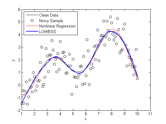
As you can see, the LOWESS curve is doing a great job capturing the dynamics of the system. We were able to generate a LOWESS fit that is almost as accurate as the nonlinear regression without the need to specify that this system should be modeled as a second order Fourier series.
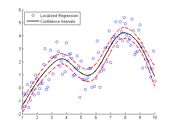
Here's a bonus for those you you who stuck around to the end. This next bit of code generates confidence intervals for the LOWESS fit using a "paired bootstrap".
scatter(X, noisy) f = @(xy) mylowess(xy,X,span); yboot2 = bootstrp(1000,f,[X,noisy])'; meanloess = mean(yboot2,2); h1 = line(X, meanloess,'color','k','linestyle','-','linewidth',2); stdloess = std(yboot2,0,2); h2 = line(X, meanloess+2*stdloess,'color','r','linestyle','--','linewidth',2); h3 = line(X, meanloess-2*stdloess,'color','r','linestyle','--','linewidth',2); L5 = legend('Localized Regression','Confidence Intervals',2); snapnow
Can anyone provide a good intuitive explanation how the bootstrap works? For extra credit:
Post your answers here.
Get the MATLAB code (requires JavaScript)
Published with MATLAB® 7.11