January 13, 2011 6:11 AM
by Loren
Data Driven Fitting
This week Richard Willey from technical marketing will be guest blogging about nonparametric fitting.
Contents
This week's blog is motivated by a common question on MATLAB Central. Consider the following problem:
- You have a data set consisting of two variables: X and Y
- You need to generate a model that the describes the relationship between the two variables
- The only thing that you have to work with is the data. You don't have any first principles information about the "true" relationship between your variables
How can you generate a curve fit that best describes the relationship between X and Y? This question traditionally shows up in in two different guises:
- Many people ask about solutions for "automatic fitting". (How can I produce a curve fit without a parametric equation?)
- The second variant involves questions about a curve fitting using high order polynomials. The user doesn't have enough "First Principles" knowledge about the system to specify a model, but does know that a 9th order polynomial can describe a very complicated system.
In this week's blog, I'm going to show you a better way to solve this same problem how to use a combination of localized regression and cross validation.
- You can access localized regression using the smooth function in Curve Fitting Toolbox
- Cross validation is available using the cvpartition function in Statistics Toolbox
Generate some data to work with
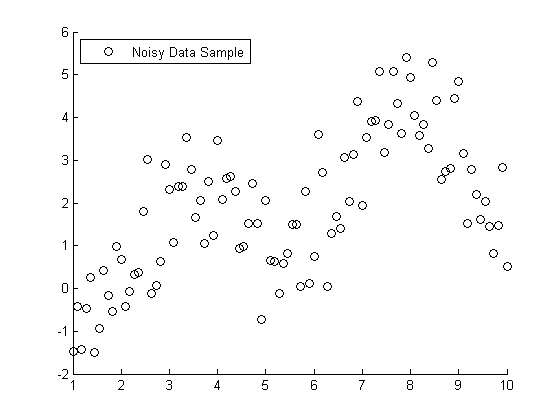
To use a more visual approach, suppose you had the following set of data points:
s = RandStream('mt19937ar','seed',1971); RandStream.setDefaultStream(s); X = linspace(1,10,100); X = X'; % Specify the parameters for a second order Fourier series w = .6067; a0 = 1.6345; a1 = -.6235; b1 = -1.3501; a2 = -1.1622; b2 = -.9443; % Fourier2 is the true (unknown) relationship between X and Y Y = a0 + a1*cos(X*w) + b1*sin(X*w) + a2*cos(2*X*w) + b2*sin(2*X*w); % Add in a noise vector K = max(Y) - min(Y); noisy = Y + .2*K*randn(100,1); % Generate a scatterplot scatter(X,noisy,'k'); L2 = legend('Noisy Data Sample', 2); snapnow

Nonlinear Regression example
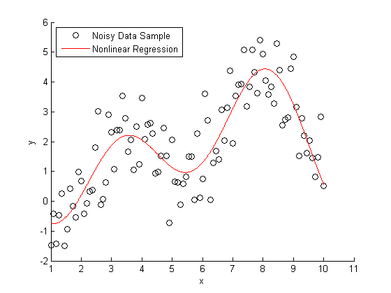
If you knew that this data was generated with a second order Fourier series, you use nonlinear regression to model Y = f(X).
foo = fit(X, noisy, 'fourier2') % Plot the results hold on plot(foo) L3 = legend('Noisy Data Sample','Nonlinear Regression', 2); hold off snapnow
foo = General model Fourier2: foo(x) = a0 + a1*cos(x*w) + b1*sin(x*w) + a2*cos(2*x*w) + b2*sin(2*x*w) Coefficients (with 95% confidence bounds): a0 = 1.734 (1.446, 2.021) a1 = -0.1998 (-1.065, 0.6655) b1 = -1.413 (-1.68, -1.146) a2 = -0.7688 (-1.752, 0.2142) b2 = -1.317 (-1.867, -0.7668) w = 0.6334 (0.5802, 0.6866)

Nonparameteric Fitting Example
All very nice and easy... We were able to specify a regression model and plot our curve using a couple lines of code. The coefficients that were estimated by our regression model are a close match to the ones that we originally specified.
Here's the rub: we cheated. When we created our regression model, we specified that the true relationship between X and Y should be modeled using a second order Fourier series. What if this information wasn't available to us?
This next piece of code is a bit more complicated, however, it will solve the same problem using nothing but the raw data and some CPU cycles.
We're going to use a smoothing algorithm called LOWESS (Localized Scatter Plot Smoothing) to generate our curve fit. The accuracy of a LOWESS fit depends on specifying the "right" value for the smoothing parameter. We're going generate 99 different LOWESS models, using smoothing parameters between zero and one, and see which value generates the most accurate model.
This type of brute force technique often runs into problems with "overfitting". The LOWESS curve that minimizes the "sum of the squared errors" fits both the signal and the noise component of the data set.
To protect against overfitting, we're going to use a technique called cross validation. We're going to divide the data set into different training sets and test sets. We'll generate our predictive model using the data in the training set, and then measure the accuracy of the model using the data in the test set.
num = 99; spans = linspace(.01,.99,num); sse = zeros(size(spans)); cp = cvpartition(100,'k',10); for j=1:length(spans), f = @(train,test) norm(test(:,2) - mylowess(train,test(:,1),spans(j)))^2; sse(j) = sum(crossval(f,[X,noisy],'partition',cp)); end [minsse,minj] = min(sse); span = spans(minj);
mylowess is a function that I wrote that estimates values for a lowess smooth. I've included a copy of mylowess.m for you to use.
type mylowess.mfunction ys=mylowess(xy,xs,span) %MYLOWESS Lowess smoothing, preserving x values % YS=MYLOWESS(XY,XS) returns the smoothed version of the x/y data in the % two-column matrix XY, but evaluates the smooth at XS and returns the % smoothed values in YS. Any values outside the range of XY are taken to % be equal to the closest values. if nargin<3 || isempty(span) span = .3; end % Sort and get smoothed version of xy data xy = sortrows(xy); x1 = xy(:,1); y1 = xy(:,2); ys1 = smooth(x1,y1,span,'loess'); % Remove repeats so we can interpolate t = diff(x1)==0; x1(t)=[]; ys1(t) = []; % Interpolate to evaluate this at the xs values ys = interp1(x1,ys1,xs,'linear',NaN); % Some of the original points may have x values outside the range of the % resampled data. Those are now NaN because we could not interpolate them. % Replace NaN by the closest smoothed value. This amounts to extending the % smooth curve using a horizontal line. if any(isnan(ys)) ys(xs<x1(1)) = ys1(1); ys(xs>x1(end)) = ys1(end); end
Evaluate the accuracy of our LOWESS fit
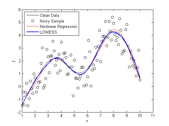
Next, let's create a plot that shows
plot(X,Y, 'k'); hold on scatter(X,noisy, 'k'); plot(foo, 'r') x = linspace(min(X),max(X)); line(x,mylowess([X,noisy],x,span),'color','b','linestyle','-', 'linewidth',2) legend('Clean Data', 'Noisy Sample', 'Nonlinear Regression', 'LOWESS', 2) hold off snapnow

As you can see, the LOWESS curve is doing a great job capturing the dynamics of the system. We were able to generate a LOWESS fit that is almost as accurate as the nonlinear regression without the need to specify that this system should be modeled as a second order Fourier series.
Special Guest Appearance by bootstrp
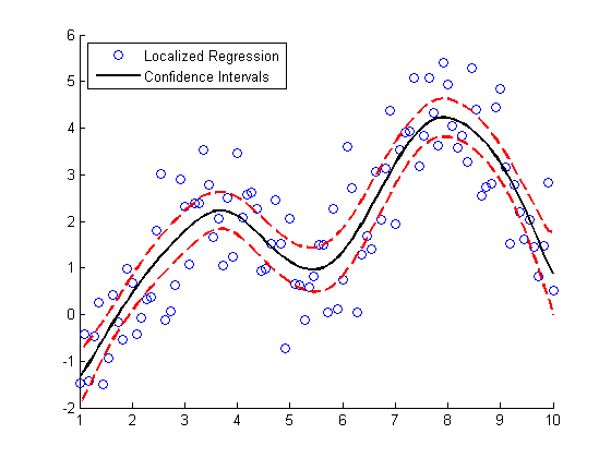
Here's a bonus for those you you who stuck around to the end. This next bit of code generates confidence intervals for the LOWESS fit using a "paired bootstrap".
scatter(X, noisy) f = @(xy) mylowess(xy,X,span); yboot2 = bootstrp(1000,f,[X,noisy])'; meanloess = mean(yboot2,2); h1 = line(X, meanloess,'color','k','linestyle','-','linewidth',2); stdloess = std(yboot2,0,2); h2 = line(X, meanloess+2*stdloess,'color','r','linestyle','--','linewidth',2); h3 = line(X, meanloess-2*stdloess,'color','r','linestyle','--','linewidth',2); L5 = legend('Localized Regression','Confidence Intervals',2); snapnow

Can anyone provide a good intuitive explanation how the bootstrap works? For extra credit:
- Can you convert this example from a "paired bootstrap" to a "residual bootstrap"?
- Do you see any advantages or limitations to the different types of bootstraps?
Post your answers here.
Get the MATLAB code (requires JavaScript)
Published with MATLAB® 7.11
Art Trembanis
No comments:
Post a Comment